This tutorial will guide you on the process of using the reverse homology webtool to explore hypotheses about an intrinsically disordered region. We will be using an IDR in the human protein hnRNPA1 as an example. If you want to follow along with this tutorial, the sequence can be copied below:
SKQEMASASSSQRGRSGSGNFGGGRGGGFGGNDNFGRGGNFSGRGGFGGSRGGGGYGGSGDGYNGF GNDGGYGGGGPGYSGGSRGYGSGGQGYGNQGSGYGGSGSYDSYNNGGGGGFGGGSGSNFGGGGSYN DFGNYNNQSSNFGPMKGGNFGGRSSGPYGGGGQYFAKPRNQGGYGGSSSSSSYGSGRRF
Alternatively, if you want to skip the processing time, you can simply navigate to this link, which contains a pre-loaded version of the output for the IDR in hnRNPA1.
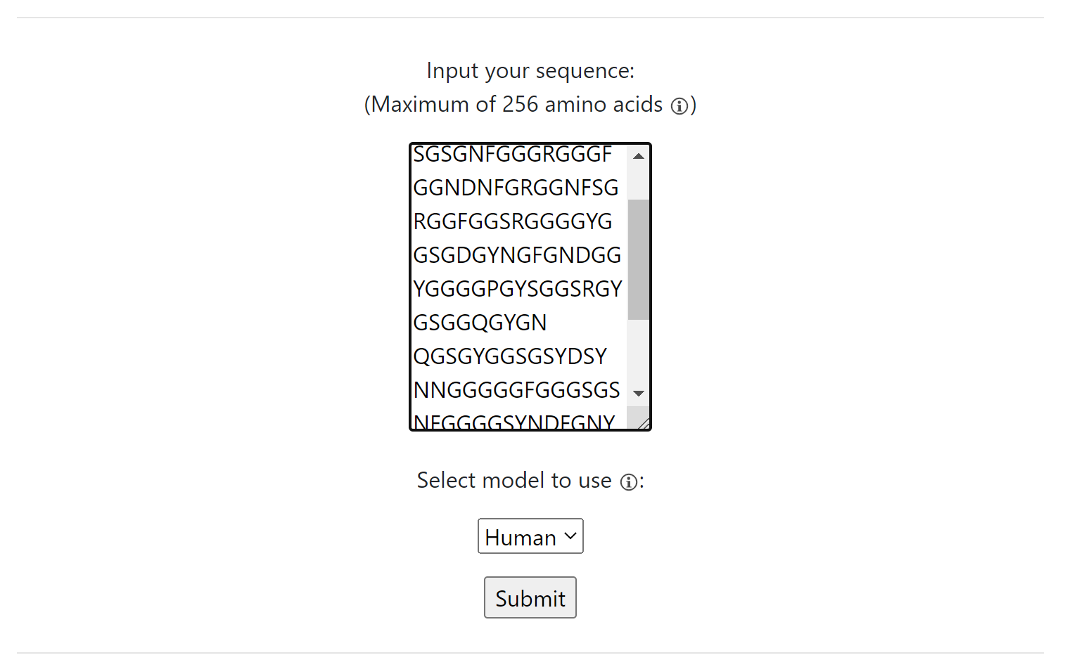
Navigate to the front page and input the sequence in the text box provided. Note that our webapp only accepts sequences up to 256 amino acids. This is the longest sequence that the neural network can handle. If you have a sequence longer than that, you have two strategies: first, you can crop up the sequence and query multiple crops. Since our neural network is not capable of modeling long-range distal interactions, cropping up a sequence like this will not radically change what kinds of features a neural network will perceive in the sequence (although this is something we might upgrade in future versions of the method.
Under "Select Model to Use", you can specify what species to use: the human model, which was trained on homologues of human IDRs across vertebrates, and the yeast model, which was trained on homologues of yeast IDRs across yeast species. Technically, any sequence can be inputted into either model. In practice, the models have differing features reflecting what kinds of features are present or more prevalent in these proteomes, so picking a model that more closely corresponds to your sequence of interest should help the model identify more relevant features in the sequence (although we have not extensively tested generalization of models on sequences of different species than the ones they were trained on.)
In our case, we will use the human model since we're working with an IDR from a human protein.

Press "submit" and grab some coffee or check your email!
Your sequence has been queued for processing by our neural network. Processing time will depend on the size of the queue and length of your sequence, but usually takes 1-5 minutes. Once your outputs are ready, you will be automatically redirected to the analysis page.
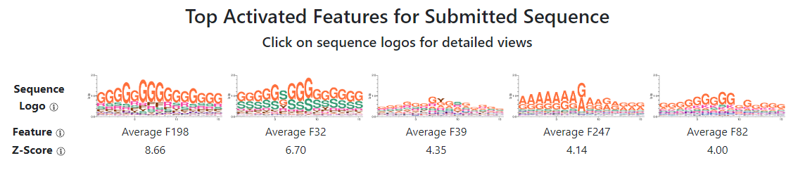
The first page of the results will show five sequence logos, corresponding to the five features the model thinks is most important to the sequence. These sequence logos represent the kinds of sequences that each neuron in our neural network generating a feature most "likes" (i.e. outputs the highest values for.) Importantly, these sequence logos are not calculated using your input sequence exclusively, but using all IDRs in the proteome. In other words, the amino acids shown in the sequence logos may not fully match subsequences in your sequence, especially since our neural network features are "flexible" and can capture different kinds of sequences in the same feature.

Sequences can either be "average" features or "max" features. Average features represent "bulk" sequence features that are distributed over the entire sequence. While they are shown as 15 residue-width sequence logos, this window is arbitrary: average features pool information from over the entire sequence, and scale linearly as more of the sequence contains that property. For example, an average sequence with a lot of D/Es would increase in value as more of the input sequence is negatively charged (D or E). In contrast, max features do look for features that occur in local 15-residue windows: these features capture properties like local motifs, recognizing a local part of a sequence that most matches the neural network feature.

For our input hnRNPA1 IDR, we can see that the top five features are all average features. This does not always happen (many times, there is a mixture of both average and max features), but our model appears to be especially sensitive to the bulk features in this particular IDR. The features contain an abundance of Gs, Ss, and As, suggesting that an abundance of amino acids with tiny sidechains distributed across the entire sequence is a distinguishing value of the hnRNPA1 IDR (although as we will see in the next step, diving down into the details of these features will reveal more subtlety.)

Finally, each feature is associated with a z-score. This z-score tells us how strong the feature is, compared to all other IDRs in the reference proteome (i.e. human or yeast.) A low z-score does not necessarily mean that the feature is not biologically relevant, but it does tell us that many IDRs also similarly active the feature, suggesting that the features identified are less distinguishing hallmarks of the input sequence, or the sequence is only a "weak" match to the feature in the neural network. In our case of hnRNPA1, we can see the z-scores are rather strong: the top feature, Average F198, has a z-score of 8.67, suggesting that it is fairly rare for IDRs to activate Average F198 as much as hnRNPA1 has.
Next, click on the sequence logo for Average F198. This will bring up an expanded view of more details about the feature.
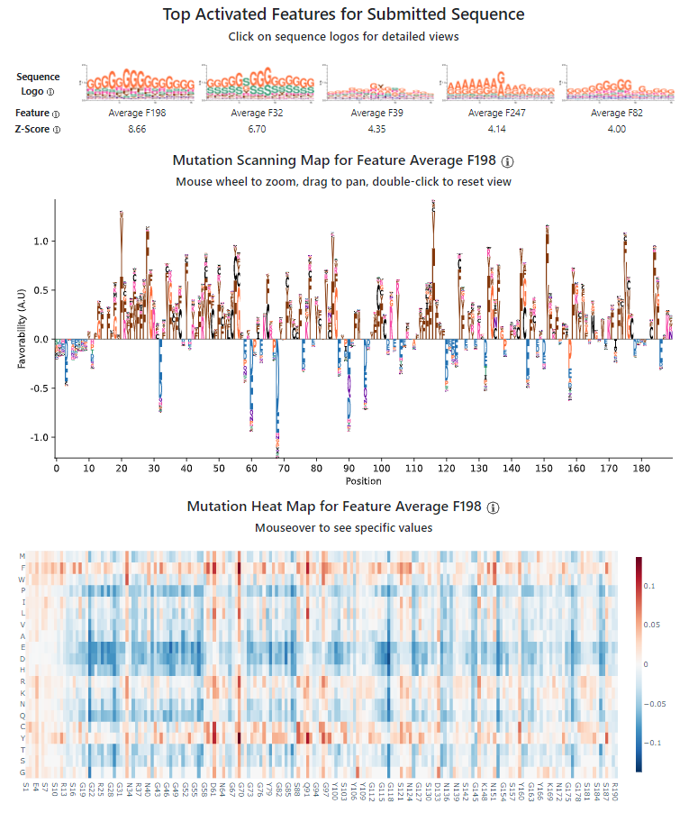
The first view you'll see is the "mutation scanning map". This is a summary that shows what amino acid positions in the wild-type position most contribute (and detract) from the feature, as well as what are the most favorable/unfavorable amino acids in the position in general. Positions with letters above the axis mean that the wild-type residue is favored over most other amino acids, while positions with letters below the axis means the wild-type residue is disfavored by that feature. For positions above the axis, we show the most favorable amino acids; for positions below the axis, we show the least favorable amino acids. Keep in mind that the most/least favored amino acids may not be the original wild-type residue: the original residue is generally favorable/unfavorable, but there may be some residues that are even more/less favorable than it. Also keep in mind that this is the view for one feature alone: usually, there are multiple features working to describe the IDR, so looking at multiple holistically can produce richer hypotheses.
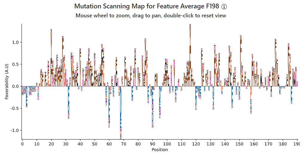
The mutation scanning map for Average F198 for our IDR in hnRNPA1 reveals a marked preference for aromatic amino acids, Y/F, in many positions. This may seem at odds with the sequence logo, but keep in mind that the sequence logo is calculated globally on all IDRs, while we are analyzing a specific IDR in this case. Aromatic amino acids tend to be pretty rare in IDRs, but are especially enriched in our hnRNPA1 IDR (as we will see in more detail in the next view.) In contrast, Gs are more common in IDRs across the proteome, and our feature is still generally favorable towards Gs (and also Rs, which are visible in the sequence logo and favored at many positions in hnRNPA1 too.) Overall, this mutation scanning map tells us that for this particular feature, aromatic amino acids occurring alongside Gs and Rs is very favorable to the feature.
We can repeat this process for the other features. Click on the sequence logo for Average F82 next.
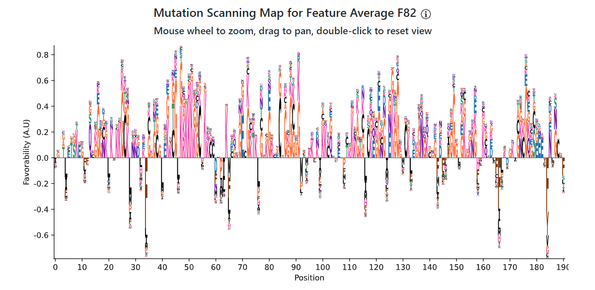
Even though the sequence logos are very similar, the mutation scanning maps show markedly different behavior between Average F198 and Average F82. While Gs and Rs are favorable to both features, Average F82 more strongly prefers positive (R/K) residues - and in fact, disfavors aromatic (and in general, hydrophobic) residues - in contrast to Average F198, which strongly favored aromatic residues. However, note that the z-score for this feature (3.98) is markedly lower than that for Average F198 (8.67). One interpretation is that while the abundance of positive residues and Gs in hnRNPA1 activate this feature, the presence of aromatic amino acids drags it down. In other words, it's possible to keep in mind that features with weaker z-scores may only partially match the biological reality of the sequence - examining multiple features holistically can help with judgment calls about how relevant features are.
Return to the expanded view for Average F198 and scroll down to the bottom of the page.

You are now looking at the mutation heat map for Average F198 for the hnRNPA1 RNA. This is a similar view to the mutational scanning map, but instead of showing a summary, it now shows the specific effect of each point mutation. Blue values show positions where replacing the wild-type amino acid with the amino acid labeled on the Y-axis would drop the value of the feature, while red values show positions where replacing the wild-type would increase it. In other words, columns with lots of blue are amino acids the model really wants to retain for that feature.
For our IDR, the mutation heat map has several strongly blue columns. We'll zoom in on some of these by clicking and dragging: let's center the map around residues 21 to 41.
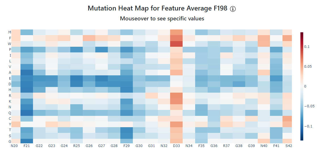
We can see from the X-axis at the bottom, that many of the strongly blue bands correspond to F - for example, F21 and F29 are especially favorable. Other favorable amino acids include G (especially from G22 to G31) - while mutating these amino acids to most other amino acids except F and Y would not drop the feature as much as mutating F21 or F29, we would still see a drop in the feature. Finally, Rs are also frequently favorable, especially F25. Interestingly, the same amino acid at different positions contribute differently to the feature: F35 is still favorable, but not as much as F21 or F29. While it is difficult to say why exactly, we can speculate that it has to do with the context: F21 and F29 are surrounded by more Gs, and form more of a continuous stretch of favorable residues.
Our method is deterministic, and will produce the same outputs each time you input the sequence (excepting version updates.) However, if you think you might run the same sequence multiple times to revisit these outputs, you might want to skip the processing time. The sequence logos and mutation scanning maps are rendered as image files, and can be saved simply by right-clicking and downloading them. The mutation heat map can be saved as a PNG by hovering, and then clicking the camera icon on the menu to "download plot as a png."